This is a special post. It is not linked to human rights or citizenship, but to data analysis and … running. Yes, I started running a lot during the pandemic as a way to deal with stressful times, including working from home and home schooling of kids etc. I never liked running much, but in the past years, I really started enjoying it. Already in 2021, I joined the marathon relay team of the Fundamental Rights Agency at the Vienna City Marathon (VCM), where I ran the first leg of 15.5 km (other team mates run about 10 km, 5.5 km and 11 km, respectively, to complete the full marathon distance). This year, in 2022, I decided to also run the half marathon. Why is that relevant for a blog on data analysis? Because I found out that there are loads of data on the website of the VCM. If you go to the website of the VCM, you will find the results of all marathons for many years. I could not let go. And here is the result.
This analysis shows the overall performance of runners, looks into correlations of factors linked to running fast (finishing times) and compares my own result to the rest of the runners. How did I perform? Was it good, bad, average? I started training in January, but had to pause in February because I overdid it in January (achillis heel), and paused training again in March because I got COVID. Luckily, I got fit again for the event and the weather was just perfect.
Data loading, cleaning and recoding
Let’s start with data collection and compilation. It is surely easy to scrape all the data from the website. However, knowing my scraping skills, while confident that I would manage, I have to admit that it would take me longer to set up a proper script, than simply copying and pasting all data into an Excel file, separately for each year. I collected data on finishing time for all VCM half marathons since 2017 for men and women of all ages from the VCM website.
Every dataset has its own challenges. The one from the VCM website is a good, relatively tidy dataset, but with some peculiarities. Let’s load and look at the data for one year.
d <- read.xlsx(paste0(pth, "vcm-hm-2022.xlsx"), sheet = 1)

# I know there is a more elegant way through the 'here' package, but I just add my path to the files in an object called 'pth'

kable(head(d))| Rang | GesRg | StNr | Name | Jahr | NAT | verein | Klasse | KlRg | Brutto | Netto |
|---|---|---|---|---|---|---|---|---|---|---|
| 0-5km | 5-10km | 10-15km | 15-20km | 20-21km | NA | NA | NA | NA | NA | NA |
| 1 | 1 | 10003 | Mario Bauernfeind | 91 | AUT | KUS ÖBV Pro | M-30 | 1 | 0.0455440 | 0.0455440 |
| 1.0729166666666666E-2 | 1.0810185185185185E-2 | 1.087962962962963E-2 | 1.0983796296296297E-2 | 2.1759259259259258E-3 | NA | NA | NA | NA | NA | NA |
| 2 | 2 | 10001 | Peter Herzog | 87 | AUT | Union Salzbu | M-35 | 1 | 0.0456134 | 0.0456134 |
| 1.0729166666666666E-2 | 1.0810185185185185E-2 | 1.0891203703703703E-2 | 1.0960648148148148E-2 | 2.2453703703703702E-3 | NA | NA | NA | NA | NA | NA |
| 3 | 3 | 20307 | Georg Schrank | 91 | AUT | Runningraz | M-30 | 2 | 0.0473148 | 0.0472685 |
Aha. This is strange. There is the header. The first row seems like a sub-header, and then there are rows that look different. The table always includes two rows per observation. The first row includes the results, name etc., and the second the split timings for every 5 km section.
OK. So, I take out the first row, which is the header of the second row, split the dataset at every second row (through adding an indicator column with alternating 1s and 2s), add proper names to the second dataset and put them back together. This is done for each year, which I loop through. Code below.
fls <- list.files(path = pth, pattern = "vcm-hm")

d <- data.frame()

f1 <- function(x) (x*1440)

nms <- c("km00t05", "km05t10", "km10t15", "km15t20", "km20t21")


for (i in fls){
  temp <- read.xlsx(paste0(pth, i), sheet = 1)
#  temp <- distinct(temp, .keep_all = TRUE)
  temp <- temp[-1, ]
  hlp <- rep(c(1,2), nrow(temp)/2)
  temp$hlp <- hlp
  d2 <- dplyr::filter(temp, hlp == 2)
  temp <- dplyr::filter(temp, hlp == 1)
  # print(paste("check", nrow(temp) == nrow(d2)))
  names(d2) <- nms
  d2 <- select(d2, all_of(nms)) %>%
  mutate_all(as.numeric) %>%
  mutate_all(f1)
  temp <- bind_cols(temp, d2)
  temp$jahr_m <- str_sub(i, 8, 11)
  d <- rbind(d, temp)
}


d <- d %>%
  distinct(Name, Jahr, Rang, Netto, .keep_all = TRUE)

# sum(duplicated(d))
The dataset has a few duplicates, which we eliminate. Then we see what kind of data/information we can get from the dataset. It includes information on age, gender, if people joined a team (this is either a running team or a team of friends or company name that is used), and nationality.
The column of interest is called ‘Netto’, the net time, which we have to transform to minutes, by multiplying by 1440, because this way the data were stored when saved in Excel (don’t ask me more about it).
count(d, jahr_m)## jahr_m n
## 1 2017 12330
## 2 2018 12560
## 3 2019 12015
## 4 2021 6974
## 5 2022 9014# d[1, ]
nrow(d)## [1] 52893# d[!duplicated(d), ] %>% nrow()
d <- d %>%
mutate(total_mins = Netto*1440) %>%
mutate(Klasse = str_replace(Klasse, "FU", "F"),
Klasse = str_replace(Klasse, "MU", "M"),
Klasse = str_replace(Klasse, "H", "25"),
name = tolower(Name),
verein = tolower(verein),
verein1 = !is.na(verein),
AT = NAT == "AUT") %>%
separate(Klasse, c("Geschlecht", "Alter"), sep = "-") %>%
mutate(david = str_detect(name, "david reichel"),
id = 1:nrow(d))Next, we look at the section times, create a separate dataset with all section times per runner, exclude those with 0, as these are erroneous, then calculate the minimum section, maximum and the ratio between the slowest and fastest section.
tmp <- d %>%
  select(id, contains("km")) %>%
  select(-km20t21) %>%
  pivot_longer(-id, names_to = "section", values_to = "time") %>%
  filter(time > 0) %>%
  group_by(id) %>%
  mutate(mi_sect = min(time, na.rm = TRUE),
         ma_sect = max(time, na.rm = TRUE),
         mn_sect = mean(time, na.rm = TRUE),
         rt_sect = mi_sect/ma_sect) %>%
  filter(time == mi_sect) %>%
  mutate(nmb = row_number()) %>%
  ungroup() %>%
  filter(nmb == 1) %>%
  select(id, fast_sect = section, ratio_sec = rt_sect)
Lastly, we add this information to the original dataset, and calculate the number of times a runner appears in the lists over the years covered, by creating a unique column with the name, birthyear (‘Jahr’), and the year of the event. Some are again duplicates, although they may also be real, as it is likely that there are runners with exactly the same name and birth year. For ease, I still exclude them (only a few).
d <- d %>%
  left_join(tmp, by = "id") %>%
  mutate(name_jahr_m = paste0(name, "_", Jahr, "_", jahr_m),
         name_jahr = paste0(name, "_", Jahr)) %>%
  group_by(name_jahr_m) %>%
  mutate(dbl = n()) %>%
  ungroup() %>%
  filter(dbl < 2) %>%
  group_by(name_jahr) %>%
  mutate(nruns = n()) %>%
  ungroup() %>%
  mutate(Geschlecht = ifelse(Geschlecht %in% c("W", "WU"), "F", Geschlecht),
         ratio_sec = ratio_sec*100)
Analysis of performance - distribution of finishing time
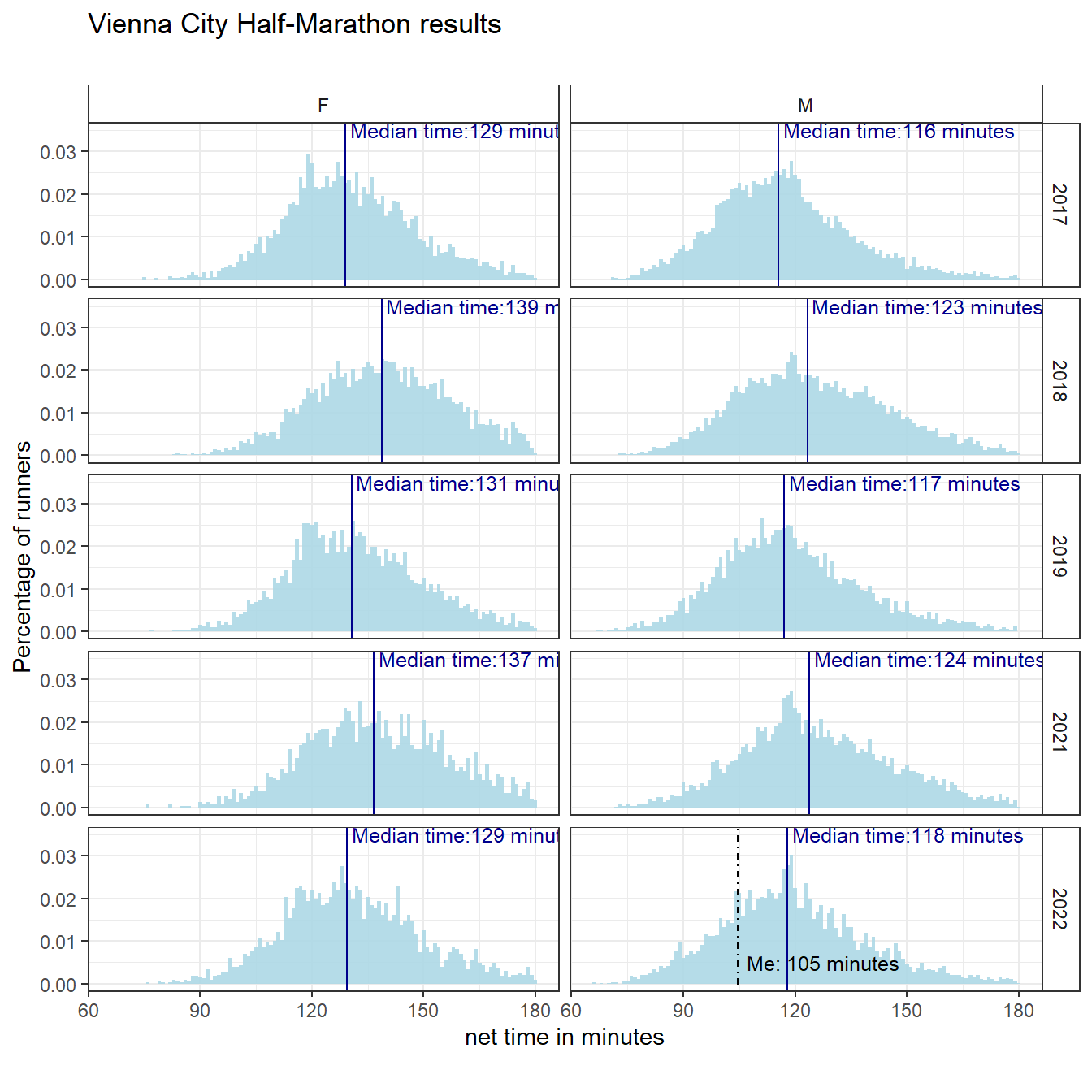
Let’s start by having a look at the distribution of all runners’ times arriving at the finishing line. The figure below shows the distribution of finishing times of all runner by gender and year of event.
smm <- d %>%
  filter(!is.na(Geschlecht)) %>%
  group_by(jahr_m, Geschlecht) %>%
  summarise(median_mins = median(total_mins),
            mean_mins = mean(total_mins)) %>%
  ungroup()
## `summarise()` has grouped output by 'jahr_m'. You can override using the `.groups` argument.drr <- d %>%
filter(str_detect(name, "david reichel"))
d2 <- filter(d, !is.na(Geschlecht))
p1 <- ggplot(d2, aes(x = total_mins)) +
geom_histogram(aes(y = ..density..), fill = "lightblue", alpha = 0.9,
binwidth = 1) +
facet_grid(jahr_m ~ Geschlecht) +
geom_vline(data = smm, aes(xintercept = median_mins), colour = "darkblue") +
geom_text(data = smm, aes(x = median_mins, y = 0.035,
label = paste0("Median time:", round(median_mins), " minutes")),
hjust = -0.02, size = 3.3, colour = "darkblue") +
geom_vline(data = drr, aes(xintercept = total_mins), linetype = 4) +
geom_text(data = drr, aes(x = total_mins, y = 0.005, label = paste0(" Me: ", round(total_mins), " minutes")), hjust = -0.02, size = 3.3) +
labs(x = "net time in minutes",
y = "Percentage of runners") +
theme_bw() +
theme(strip.background = element_rect(fill = "white")) +
labs(title = "Vienna City Half-Marathon results",
subtitle = "",
caption = "")
overall_md_time <- median(d$total_mins, na.rm = TRUE) %>% round()
overall_mn_time <- mean(d$total_mins, na.rm = TRUE) %>% round()The figure below shows the results. We see the finishing time in minutes is nicely normally distributed (sort of). I would love to encounter such beautiful distributions more often in the social sciences.
The grand overall median time is 124 minutes and the average time is 125 minutes. In the figure we can see differences over the years (likely linked to number of starters and weather conditions). 2017 was the fastest year, closely followed by 2022 (for women it was the same actually).
With the data at hand we can actually look into some factors that influence the results. In addition to the year of the race and gender, we have information on age, nationality of runner, whether the person indicated to run for a team, how often a runner joined the marathon (in the years of observation). Based on the this information, we can predict the expected time of each of the runners. I can thus predict my own performance, based on these attributes. Here it is:
########## Regression

d2 <- d %>% select(total_mins, Geschlecht, Alter, AT, verein1, name, jahr_m, nruns,
ratio_sec, fast_sect) %>% na.omit()

m1 <- lm(total_mins ~ Geschlecht + Alter + AT + verein1 + factor(nruns) + factor(jahr_m),
         data = d2)

d2 <- d2 %>%
  mutate(predicted = round(predict(m1), 1))

t1 <- d2 %>% group_by(jahr_m) %>%
  mutate(med_time = round(median(total_mins), 1)) %>%
  ungroup() %>%
  filter(str_detect(name, "david reichel")) %>%
  select(name, jahr_m, total_mins, predicted, med_time) %>%
  mutate(total_mins = round(total_mins, 1))

kable(t1, col.names = c("Name", "Year", "Time in minutes",
"Expected time based on selected variables", "Median of all runners"))| Name | Year | Time in minutes | Expected time based on selected variables | Median of all runners |
|---|---|---|---|---|
| david reichel | 2022 | 104.6 | 120.2 | 121.9 |
Wow. I did great. The expected time based on age, gender and the other charactistics mentioned above was 120.2 minutes, but I finished already after 104.6 minutes. (you see, in the end it is just a blog post about showing off)
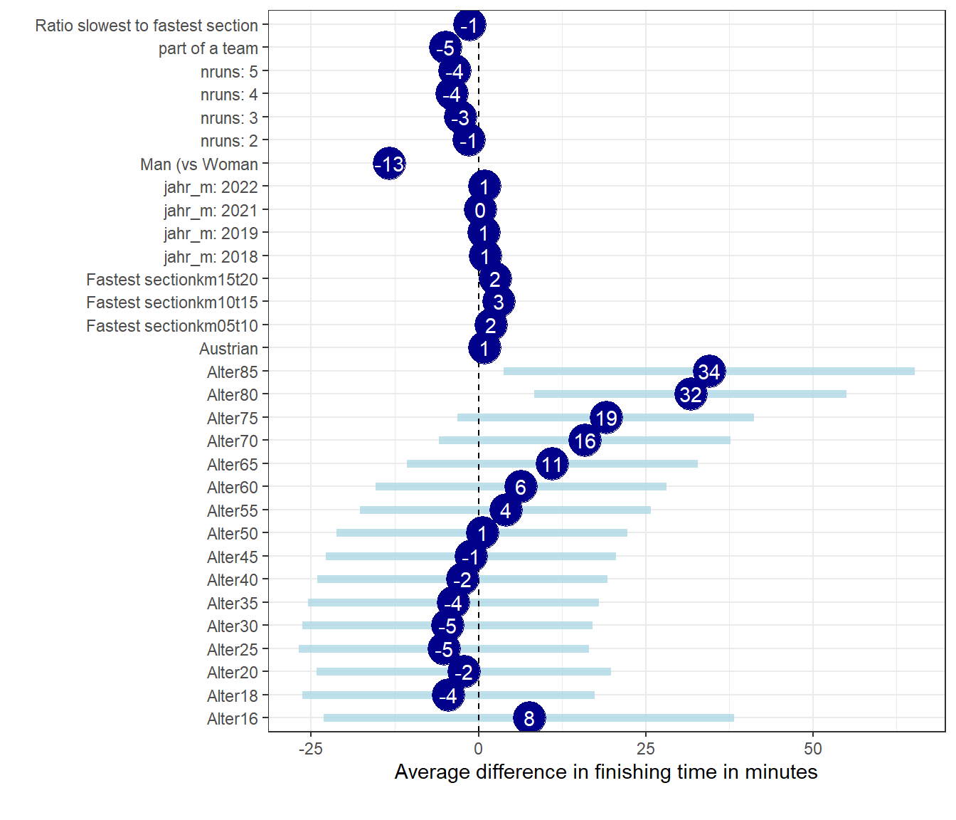
Now, let’s try to see how the factors at hand allow us to get insights into what is relevant for running fast. I run another regression, including, as above, gender, age, nationality (whether Austrian or not), team or not, how many times in the dataset, year of event (fixed effect), which of the 5 km sections was the fastest and the ratio of the fastest to the slowest section. This is not based on any scientific knowledge, but just what I thought is interesting and may be relevant (apologies to any serious scientists seriously looking into runners’ performances).
With the variables included we can explain about 39 percent of the variation in finishing times, which is quite ok. Of course, much of the explanation comes from the two new variables, about fastest section and the ratio of slowest to fastest section, which are both data from the actual run.
What do we learn? Fastest runners run the first section fastest (however, that’s anyway the case for the vast majority of runners). The higher the ratio of the fastest to the slowest 5 km section the faster you are. This means actually that the section times were relatively similar for good runners and there was not much difference between the slowest and fastest section, meaning that - as we know - good runners can run at a very stable pace throughout the entire race.
Those indicating to be part of a team are on average 5 minutes faster. Austrian nationals are on average 1 minutes slower (no surprise, many amateur runners join just for fun, and that’s good). Compared to the first time of running the halfmarathon (during the years covered), the fourth and fifth are usually faster by 4 minutes, the third by 3, and the second by one minute (all compared to the first).
All factors considered, 2017 was on average the fastest race.
Men run on average 13 minutes faster than women. And lastly, there is not much significant difference across ages, fastest around 25 and 30, slowest at 80 and 85 plus.
That’s it. Hope you liked it. Looking forward to next year. I may just indicate a team when registering for the event and hence will run 5 minutes faster … right?